By Bob Flisser, bob@swschool.com

Using an array formula to attach an IF to a function that doesn’t have one.

In a previous post, I showed how you could use an array formula to simulate an IF function that has two conditions. But arrays can create other types of what-if analysis, too.

You may know that in addition to the SUM function to add numbers, the SUMIF function will add numbers only if a condition is met. And in addition to the AVERAGE function, the AVERAGEIF function will calculate an average only if a condition is met.

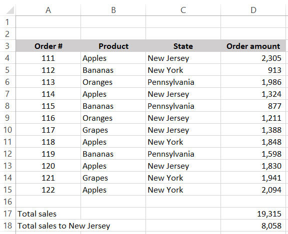
Using the example from my previous post, let’s say you’re a fruit wholesaler who is expanding into three new states. Below is a list of orders. While SUM will give you the total of all orders from all states, here’s how SUMIF will let you, uh, cherry-pick just the orders from New Jersey. Perhaps Jersey has a competitive market and you need to keep track of it.

The syntax is:

=SUMIF(range that has condition to test, the condition itself, the range of numbers to add)

In D18, the formula is (not case-sensitive):

=SUMIF(C4:C15,”new jersey”,D4:D15)

Note that since the condition is text and not a number, it has to be in quotes.

If you want to find the average of all sales to New Jersey, just replace SUMIF with AVERAGEIF.

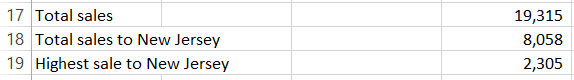
But what if you want to find the highest or lowest sale to New Jersey? Excel doesn’t have a “MAXIF” or “MINIF” function. That’s where an array formula comes to the rescue.

In D19, we’ll run the MAX function with the IF function nested in it, and enter the formula as an array. Type this formula:

=MAX(IF(C4:C15=”new jersey”,D4:D15))

Tip: when you nest one function inside another, only the outer-most function gets an equal sign before it.

…and make sure to press Ctrl + Shift + Enter. If you press Enter by itself, Excel will throw a #VALUE error.

The result is 2,305:

This says to look down column C, and wherever it finds New Jersey, add the number next to it in column D. Also notice that this IF function has a condition parameter and a True parameter, but no False parameter. It isn’t necessary, because it’s just a zero value. But if it’s easier to understand, you can get the same result if you change the formula to:

=MAX(IF(C4:C15=”new jersey”,D4:D15,0))

Now it’s your turn: in D20, find the lowest sale to New York. Download if.xlsx to get a head start.