By Bob Flisser, bob@swschool.com
Use an array formula to create an IF statement that has two conditions
The IF function in Excel lets a cell display one of two possible values, depending on whether a condition is true or false. The syntax is:
=IF(condition to test, value if the condition is true, value if the condition is false)
Note that whenever a function has multiple arguments, you separate them with commas.
For example, let’s say you’re having a sale, and want to apply a discount based on the order amount, which is in B5. If B5 is less than 100, you want B6 to show a discount amount of 6%, and if B5 has a value that’s 100 or higher, you want B6 to show a discount amount of 8%. You would enter this into B6 to display the correct percentage:
=IF(B5<100,6%,8%)
That’s a great feature, but what if you want to test for two conditions? For example, let’s say you’re a produce wholesaler and are expanding into new territory. You’re now selling different types of fruit to customers in multiple states, and you want to know if you’re making enough sales to New Jersey, which has a competitive apple market. So when looking at your sales figures, you want to add only the sales of apples to New Jersey, but not apples to New York, or bananas to New Jersey. Unfortunately, the IF function can’t do that. But don’t despair! You can use an array formula to get what you need.
With an array formula, rather than calculating values of individual cells, you calculate the values of multiple cells (a range) at once. What’s also different about array formulas is that you must enter them by pressing Ctrl + Shift + Enter, rather than just the Enter key, by itself.
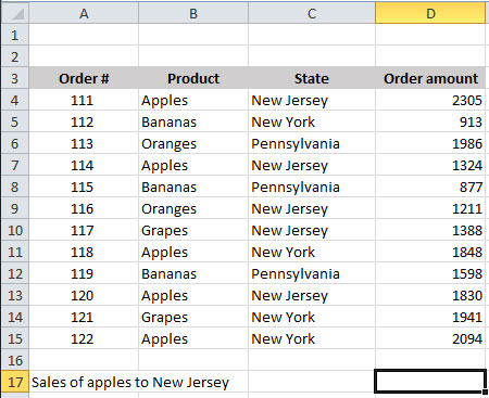
Here is a list of orders we received. We’ll put the array formula in D17.


Type this into D17 (not case-sensitive):
=SUM((D4:D15)*(B4:B15=”apples”)*(C4:C15=”new jersey”))
This formula tells Excel to use the SUM function on column D, but only in the rows where columns B and C meet your criteria for fruit and state. Since the criteria are text and not numbers, you need to put them in quotes.
After typing the formula, make sure to press Ctrl + Shift + Enter, or Excel will throw a #VALUE error.
The result in D17 should be 5459, since it doesn’t include order #118 or #122, which are for different states. Also look at the formula bar:
![]()
![]()

Excel appended curly braces { } to the beginning and end. That’s how you know it’s an array formula. If you’re a good typist, resist the temptation to type the braces yourself. It won’t work.
Think you got it? On your own, go to D18 and calculate the sales of bananas to Pennsylvania. Download multiple criteria.xlsx for a head start.